
Komanawa Groundwater Detection Power Calculator#
NOTE: while this repo was designed for groundwater calculations it is applicable to surface water as well you just have to consider the assumptions around MRT in the surface water. Typically N-NO3 for instance will be dominantly from base flow, which is often sourced from groundwater.
This package is designed to calculate the statistical power of detecting a change in groundwater/surface concentration depending on sampling duration, sampling frequency, ‘true’ receptor concentration and the noise in the receptor. there is also support for understanding statistical power in the context of groundwater travel times (e.g. lag) and groundwater temporal dispersion (e.g. mixing of different aged waters via a binary piston flow lag model).
Python Package usage#
In addition to the documentation, we have create a repository with a number of worked examples in Jupyter notebooks This repo is available at Komanawa-Solutions-Ltd/komanawa-gw-detect-power-worked-examples.
Supporting Documents#
We have included a number of supporting documents:
Water Quality Monitoring for Management of Diffuse Nitrate Pollution: This document provides guidance on the design of water quality monitoring programs for the management of diffuse nitrate pollution. It includes a section on statistical power and the use of the detection power calculator as well as other factors that should be considered when designing a water quality monitoring program.
Webinar (2024-02-19)#
On the 19th of February 2024 we held a webinar on the detection power calculator. The slides from the webinar are available in this repo and a condensed version of the talk is available on youtube.
Installation#
This package is currently held as a simple github repo, but the intention is to make it available on PyPI in the future, It also sources other repos that are only hosted on github. Therefore, the easiest way to install is to use pip and install directly from github. This will ensure that all dependencies are installed.
Install from PyPI#
pip install komanawa-gw-detect-power
Install from Github#
conda create -c conda-forge --name gw_detect  python=3.11 pandas=2.0.3 numpy=1.25.2 matplotlib=3.7.2 scipy=1.11.2 pytables=3.8.0 psutil=5.9.5
conda activate gw_detect

pip install pyhomogeneity
pip install git+https://github.com/Komanawa-Solutions-Ltd/komanawa-kendall-stats.git
pip install git+https://github.com/Komanawa-Solutions-Ltd/komanawa-gw-age-tools
pip install git+https://github.com/Komanawa-Solutions-Ltd/komanawa-gw-detect-power
Dependencies#
pandas>=2.0.3
numpy>=1.25.2
scipy>=1.11.2
tables>=3.8.0
psutil>=5.9.5
Optional Dependencies#
pyhomogeneity (for the Pettitt test)
komanawa-kendall-stats (for the Mann Kendall / MultiPart Mann Kendall / Multipart Seasonal Mann Kendall)
komanawa-gw-age-tools (for the binary piston flow lag)
Key definitions#
In this repo we have a couple key definitions:
Receptor: The receptor is the location where the concentration is measured. This is typically a groundwater well, stream or lake.
Source: The source is the location where the concentration is changed. This is typically a point source (e.g. a wastewater treatment plant) or a non-point source (e.g. a catchment/groundwater source area).
Noise: here by noise we include the variation in the concentration at the receptor. This includes true sampling noise, but also includes any other variation in the concentration at the receptor that cannot be identified or corrected for (e.g. from weather events etc.). Typically the noise will be estimated as the standard deviation of the receptor concentration time series (assuming no trend), or the standard deviation of the residuals from a model (e.g. linear regression) of the receptor concentration time series.
True Receptor Concentration: The true receptor concentration is the concentration at the receptor if there was no noise.
High Level suggested detection power methodology#
The suggested methodology for calculating the detection power of a site is as follows:
Access and review the historical concentration data and review and potentially remove outliers
(optional) if possible you may deconstruct the historical data to remove influences of seasonal/annual/inter-annual cycles, weather events etc.
Ascertain whether or not the historical concentration data has a statistically robust trend (e.g. via a Mann-Kendall test)
Estimate the noise in the receptor concentration time series a. If the historical concentration data has a statistically robust trend, then the noise can be estimated as the standard deviation of the residuals from a model (e.g. a linear regression or Sen-slope/ Sen-intercept). b. If the historical concentration data does not have a statistically robust trend, then the noise can be estimated as the standard deviation of the receptor concentration time series.
Gather data to inform the groundwater age distribution of the site. For instance a MRT and parameters for a binary piston flow lag model.
Estimate the source concentration from the historical trend (if any) and the groundwater age distribution.
Define the reduction expected in the source concentration over the implementation period to create a “once and future source concentration time series”.
Predict the true receptor concentration time series (e.g. the concentration at the receptor if there was no noise) based on the “once and future source concentration time series” and the groundwater age distribution.
Resample the true receptor concentration time series to the desired sampling frequency and duration.
Estimate the statistical power of detecting the change in concentration based on the predicted true receptor concentration time series and the noise in the receptor concentration time series.
Look up tables for statistical power#
We have included a number of lookup table to support less computationally savvy users. These look up tables are here to give estimates of the detection power.
These tables have been run for a no lag scenario with:
5, 10, 20, 30, 50, 75, & 100 year implementation times
5, 10, 15, 20, 25, 30 & 50 year monitoring durations
1, 4, 12, 26 & 52 samples/year sampling frequencies
0.05, 0.1, 0.2, 0.3, 0.4, 0.5, 0.75, 1.0, 1.5, 2, 2.5, 3, 4, 5, & 7.5 mg/l N-NO3 Noise levels
4, 5.6, 6, 7, 8, 9, 10, 11.3, 15 & 20 mg/l starting N-NO3 concentrations
5, 10, 15, 20, 25, 30, 40, 50 & 75% reductions in N-NO3 concentrations over the implementation period
The piston flow lag includes mean residence times of 1, 3, 5, 7, 10, 12, 15 years.
To use these tables:
- Locate and download the right table (decision tree):
- if you are interested in the effect of lag, then download the table for the appropriate implementation time:
open the table in a spreadsheet program (e.g. excel)
- Locate the row that corresponds to the closest:
sampling duration (samp_years)
sampling frequency (samp_per_year)
implementation_time
initial_conc
target_conc
percent_reduction
mean residence time (mrt (if applicable))
The provided power is the percent chance of detecting the change in concentration
Methodology (slope detection)#
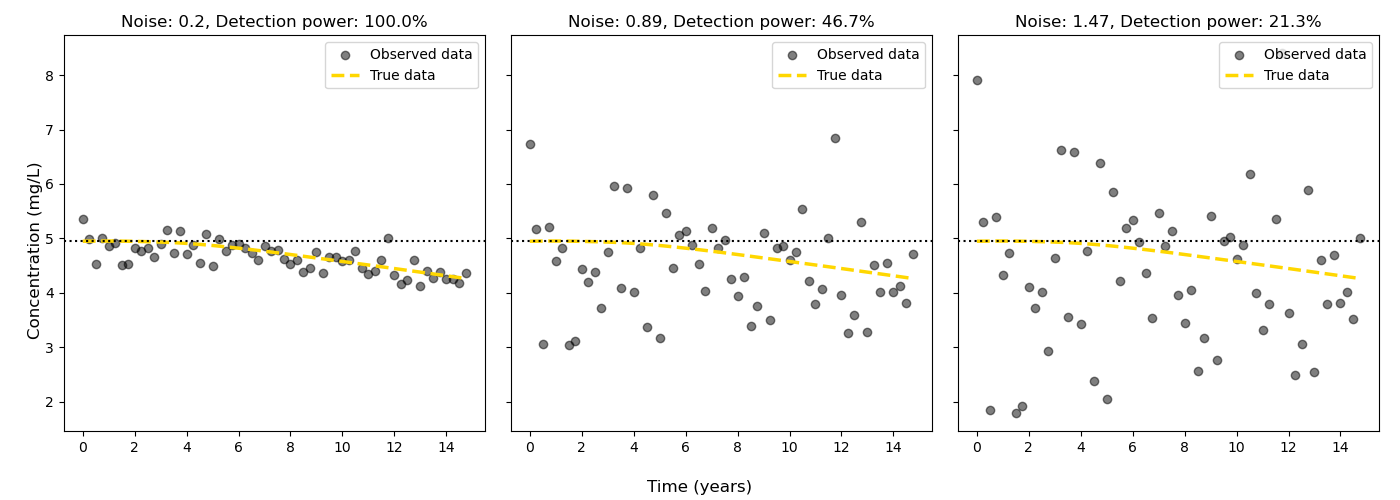
The statistical power calculation is fairly straight forward. the steps are:
Create a ‘True’ receptor time series (e.g. the concentration at the receptor/well if there was no lag)
Generate noise based on the user passed standard deviation (‘error’ kwarg). A normal distribution is used.
Add the noise to the true receptor time series
Assess the significance of the noisy receptor time series.
If the change is statistically significant (p< minimum p value) and in the expected direction, then the detection power is 1.0, otherwise it is 0.0
Repeat steps 2-5 for the number of iterations specified by the user (‘n_iterations’ kwarg) the statistical power is then reported as the mean of the detection power over the number of iterations (as a percentage).
Options to assess the significance of the noisy receptor time series#
These are listed in the order of increasing computational cost.
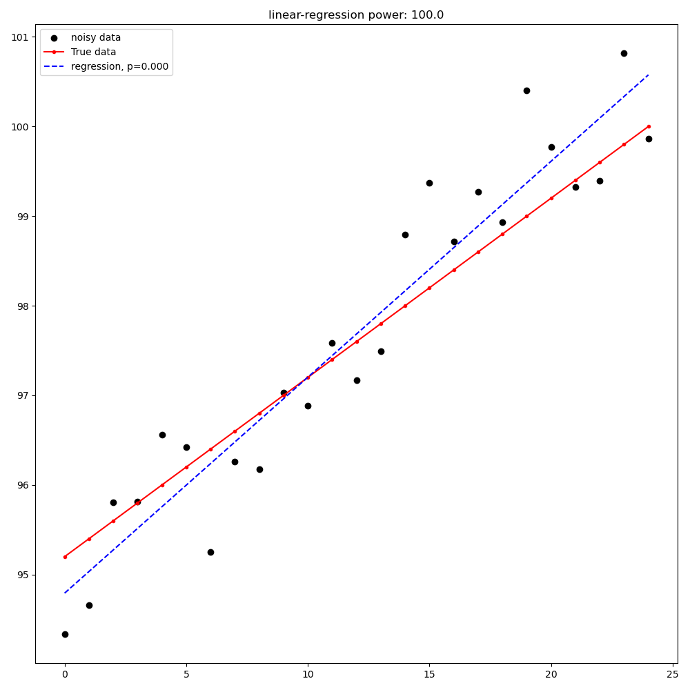
Linear regression from the first point to the last point (detection is a significant slope in the expected direction)
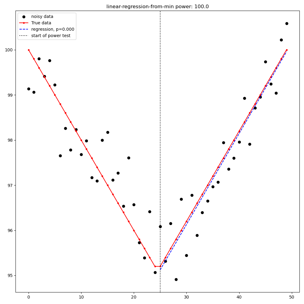
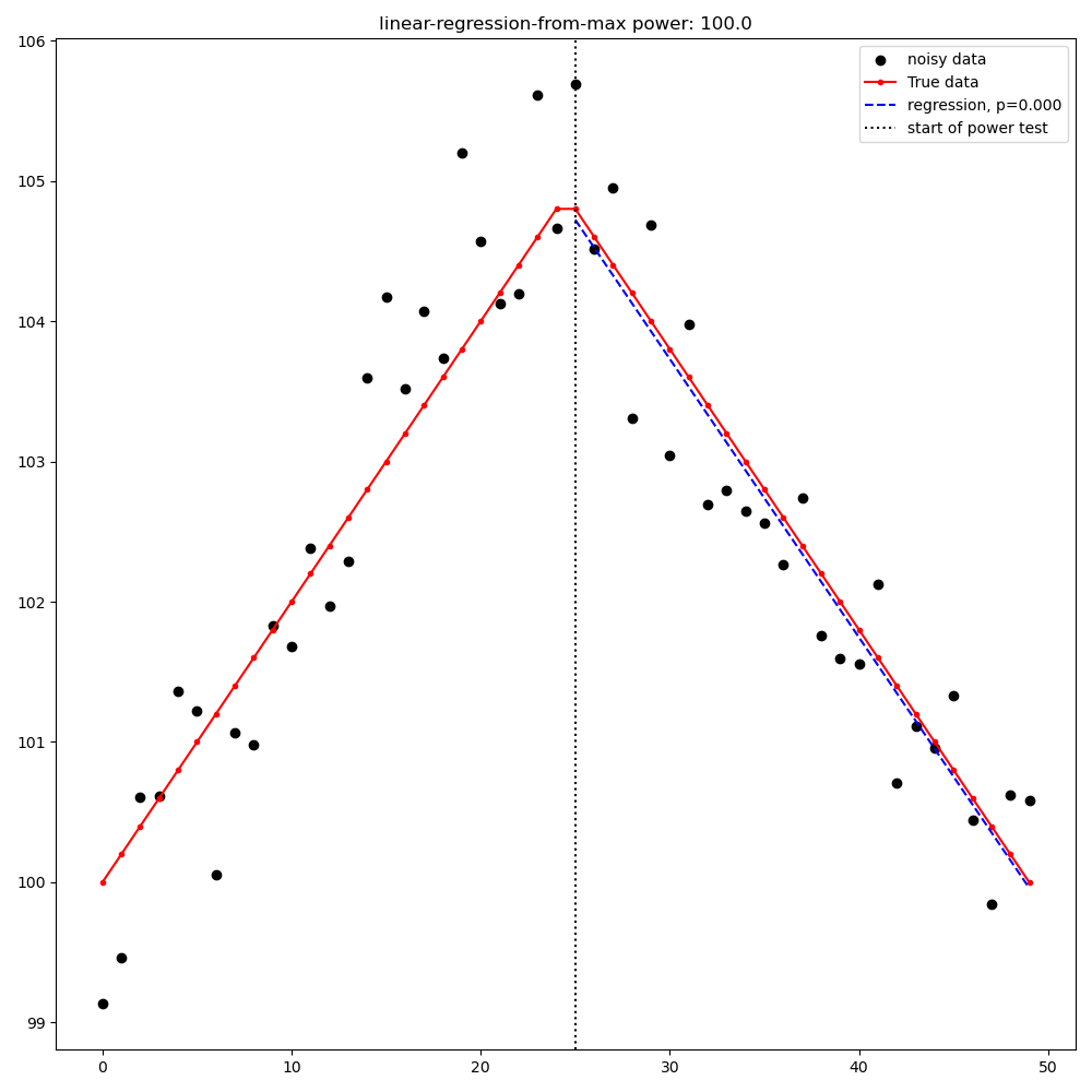
Linear regression from the [max|min] point to the last point (detection is a significant slope in the expected direction)
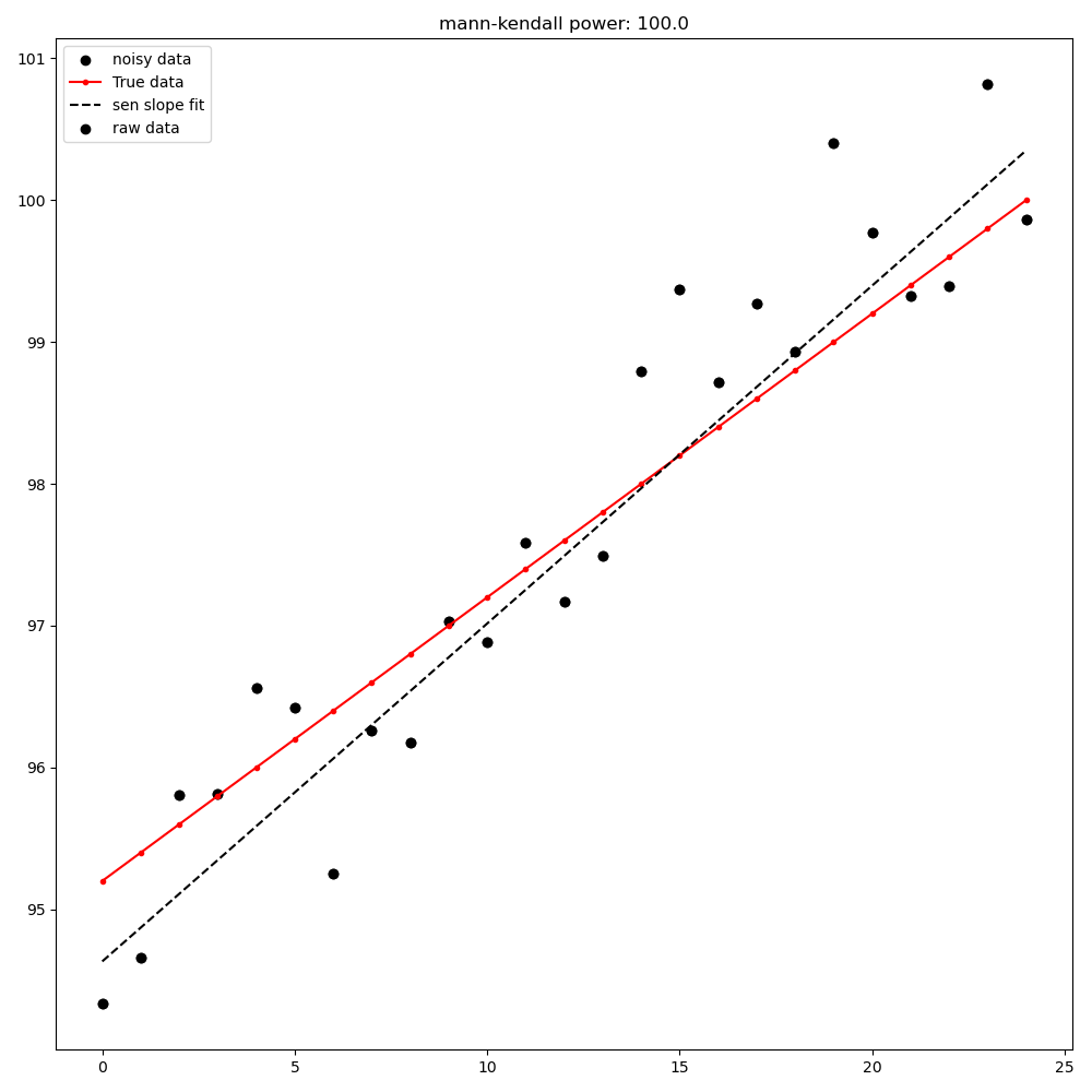
Mann-Kendall test from the first point to the last point (requires komanawa-kendall-stats optional dependency) (detection is a significant slope in the expected direction)
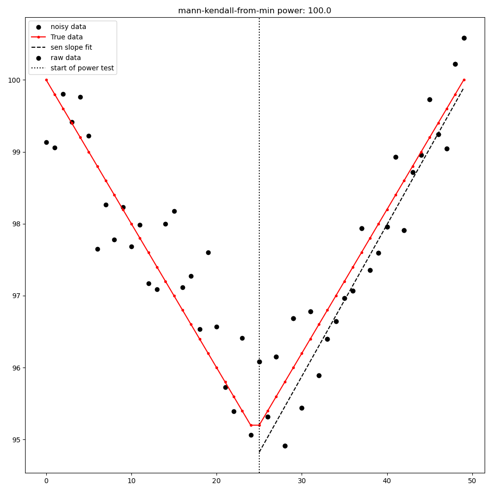
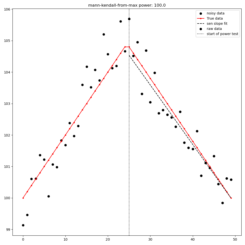
Mann-Kendall test from the [max|min] point to the last point (requires komanawa-kendall-stats optional dependency) (detection is a significant slope in the expected direction)
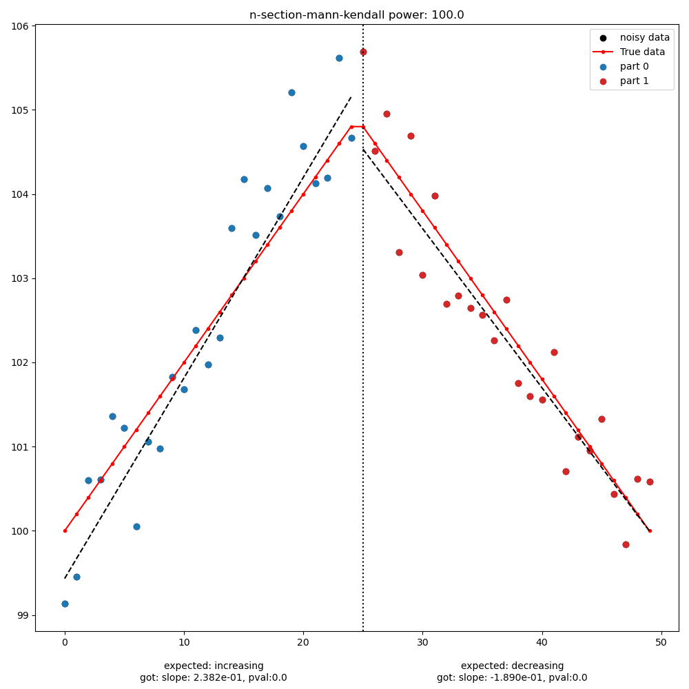
MultiPart Mann Kendall/Multipart Seasonal Mann Kendall (requires komanawa-kendall-stats optional dependency) here if the process identifies any significant breakpoints (within the alpha, no_trend_alpha, and expected slopes) the test records detection. See komanawa-kendall-stats for more details
Pettitt test (requires pyhomogeneity optional dependency)#
The pettitt test is much better a identifying step changes in the data rather than slow decreases in concentration. This can cause unexpected behaviour as compared to the other change detection tests. As an example see the figure below:

Based on this we do not suggest using the Pettitt test in conjunction with the lag models, which are designed to identify slow decreases in concentration. However, the Pettitt test is included for completeness.
Note that the pettit test requires an additional parameter nsims_pettit. This is the number of simulations to run to estimate the p value. The default is 2000, but this can be increased to improve the accuracy of the p value or decreased to reduce the computational burden. in support the run times of a single pettitt test (recall it will be run self.nsims times) is shown below:
2 pettitt simulations: 8.0e-4 seconds
20 pettitt simulations: 3.0e-3 seconds
200 pettitt simulations: 2.5e-2 seconds
2000 pettitt simulations: 2.4e-1 seconds
20000 pettitt simulations: 2.5 seconds
the effect on the pvalue is shown in the figure below:

Methodology (Counterfactual)#
The counterfactual methodology is similar to the slope methodology, but instead of assessing the significance of the slope it assesses the significance of the difference between the true receptor concentration time series and the noisy receptor concentration time series.
We have implemented the following significance tests:
Paired t-test
Wilcoxon signed rank test
Resource Requirements (slope)#
NOTE: we have not assessed the resource requirements for the counterfactual methodology as they are significantly lower than the slope methodology.
The Detection power calculator can use substantial resources depending on the number of iterations and the significance mode used. In general the significance mode efficiency is as follows:
Linear regression based techniques
Mann-Kendall based techniques
Pettitt test
MultiPart Mann-Kendal
We have implemented an efficiency mode to decrease the computational resource requirements. The effect of the mode depends on the significance test
For linear regression and Mann-Kendall techniques the efficiency mode first calculates the pvalue and sign for the true (noise free) concentration time series. If the pvalue is greater than the minimum pvalue then the power is set to 0.0 and the power calculations are not run on the noisy concentration time series. This can significantly decrease the computational resource requirements.
For the MultiPart Mann-Kendall efficiency mode both calculates the trend detection on the true time series (and then returns a power of 0 if the trend is not detected) and reduces the number of possible breakpoints that are assessed by creating a possible window to test each breakpoint. This window is defined by the maximum of:
the minimum number of breakpoints to test (mpmk_efficent_min)
or as a fraction of the length of the full time series (mpmk_window).
Note that you can also and independently set the step size of the breakpoints (mpmk_check_step) (e.g a step size of 1 will test every possible breakpoint, a step size of 2 will test every second breakpoint etc.). For more information see the docstring, the docstring of the MultiPartMannKendall class, and the komanawa-kendall-stats repo. Where both a mpmk_window and a check_step>1 is passed the mpmk_window will be used to define the window size and the check_step will be used to define the step size within the window. The minimum number of breakpoints to test (mpmk_efficent_min) is always respected (i.e. if the window size is less than the minimum number of breakpoints to test, then the window size will be increased to the minimum number of breakpoints to test, but the space between breakpoints will still be defined by check_step).
For the Pettitt test the efficiency mode is not yet implemented.
Memory Requirements#
For linear regression techniques the memory requirement is relatively minor
For mann-kendall techniques the memory requirement is proportional to the number of samples in the time series. For all Mann-Kendall techniques the program must calculate the “s_array” which is the difference between all pairs of samples. The s_array is a square matrix with the number of rows and columns equal to the number of samples in the time series. Therefore the memory requirement is:
N: 4 * s_array memory
50: 8e-05 gb
100: 0.00032 gb
500: 0.008 gb
1,000: 0.032 gb
5,000: 0.8 gb
10,000: 3.2 gb
25,000: 20.0 gb
50,000: 80.0 gb
We have not assessed the Pettitt test memory requirements.
Example Runtimes#
The following table shows the run time for a single iteration of the power calculation for each significance mode. Note that the resource requirements are for a single threaded process. The table of processing times was run on a single thread (11th Gen Intel(R) Core(TM) i5-11500H @ 2.90GHz with 32 GB of DDR4 RAM). The results are in seconds. For these tests we set the following variables:
# constants
nsims = 10
mpmk_check_step = 1
mpmk_efficent_min = 10
mpmk_window = 0.05
nsims_pettit = 2000

# iterables
methods = DetectionPowerCalculator.implemented_significance_modes
ndata = [50, 100, 500, 1000, 5000]
efficency_modes = [True, False]
If you want a processing time table for a different machine run:
from pathlib import Path
from komanawa.gw_detect_power.timetest import timeit_test
data = timeit_test()
data.to_csv(Path.home().joinpath('Downloads', 'timeit_test_results.txt'))
Note that this may take some time
linear regression techniques#
n data |
linear-regression |
linear-regression-from-max |
linear-regression-from-min |
|---|---|---|---|
50 |
1.01E-03 |
8.62E-04 |
8.33E-04 |
100 |
1.03E-03 |
8.91E-04 |
8.74E-04 |
500 |
1.28E-03 |
1.11E-03 |
9.72E-04 |
1000 |
1.26E-03 |
1.10E-03 |
1.10E-03 |
5000 |
2.69E-03 |
2.03E-03 |
2.01E-03 |
Mann-Kendall Techniques#
n data |
mann-kendall |
mann-kendall-from-max |
mann-kendall-from-min |
|---|---|---|---|
50 |
3.45E-03 |
3.26E-03 |
3.20E-03 |
100 |
3.82E-03 |
3.32E-03 |
3.33E-03 |
500 |
1.27E-02 |
5.70E-03 |
5.44E-03 |
1000 |
5.82E-02 |
1.31E-02 |
1.25E-02 |
5000 |
1.58E+01 |
1.79E+00 |
1.79E+00 |
MultiPart Mann-Kendall / Pettitt test#
n data |
efficency_mode |
n-section-mann-kendall |
pettitt-test |
|---|---|---|---|
50 |
True |
5.71E-02 |
na |
50 |
False |
9.27E-02 |
8.91E-01 |
100 |
True |
6.92E-02 |
na |
100 |
False |
2.38E-01 |
9.36E-01 |
500 |
True |
3.95E-01 |
na |
500 |
False |
1.80E+00 |
1.35E+00 |
1000 |
True |
1.22E+00 |
na |
1000 |
False |
5.91E+00 |
1.83E+00 |
5000 |
True |
1.21E+02 |
na |
5000 |
False |
5.47E+02 |
5.88E+00 |
Example plots for each significance mode (slope)#
Linear Regression from first point to last point#
Linear Regression from [max|min] point to last point#
Mann-Kendall test from first point to last point#
Mann-Kendall test from [max|min] point to last point#
MultiPart Mann Kendall test#
Pettitt test#

Further Improvements#
If you have any suggestions for improvements please let us know by raising an issue on the github repo.